Coordinates from arrays and surfing in MatLab

So I've been embarking on a mission to make a good, conceptual model of hill slope ecosystem processes that define productivity. I've got a model that describes some of these processes already and it's pretty useful, but right now playing with it is pretty hard because it invokes a lot of details that are beyond the current (basic) scope of what I'm thinking of.

So I decided that I would take the pre-processed DEM file from that model (processed to allow downhill percolation) and specifically the part cut to the boundaries of my watershed, and start to play with it.

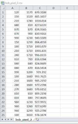
One challenge was that I essentially had the data in a format that was 3 vectors (columns) of x-axis location, y-axis location, and z-axis locations. I had no idea how to process this, so I asked my husband who wrote me a script and then kindly explained it to me.

Here's the original file:

My file is called "ws1_elev" which you can see below how it is imported here:

so first, he created two variables, "data" which is essentially the same as "ws1_elev" and "N" which is the length of the data (I believe it was something like 1151 rows long).

Now, my x and y coordinates were on a 30 x 30 m scale, and since I wanted to look at this as a picture, that would not be convenient for here. I would have just one point every 900 square meters. So we divided the x and y coordinates by 30 by saying:

data( : , 1 : 2) = data ( : , 1 : 2) / 30 + ones (length (data) , 2) ;

in short, in the new matrix "data", all rows (: ,) of the first two columns (1 : 2) are the same as those rows divided by 30 ( /30). We then add "one" to every unit in the second column because otherwise many of these units would be "0" and MatLab does not like 0's in its arrays.

Now, we want to tell it to understand that these first two columns are actually coordinates. So here's the brilliance,  create a matrix of zeros as big as the maximum length in columns 1 and  2 (essentially think of this as making a piece of grid paper as big as your coordinates) 

A = zeros (max (data (: ,1)), max(data(:,2)));

now, for every account in your original matrix (there are N of them)

for i = 1:N 

A(data(i,1), data(i,2)) = datai3);

end

What is this doing? I didn't know, so he explained, and now I will share...
Well think of if you had a matrix in Matlab named "B." B is a matrix of random numbers drawn from the normal distribution:

Now, if you wanted to look at that component there, -0.1935, you see that, it's in the 2nd row and second column, so it's coordinates (location) are (2,2). You are calling it from "B" so call it B(2,2)

So that's what you are doing here, you are saying that the matrix A is defined by coordinates at data(:,1) and data (:,2). Furthermore, those coordinates have a specific "z-value" associated with them (in this case, it's ACTUALLY a z-value, elevation) which is stored in data (:,3). Two birds with one stone!

Now, I want to look at this matrix. And by look at it I don't mean just look at a giant array of numbers. I want it to look nice. I could use Plot3 and look at the three columns of "A" but that's just going to look bad. So instead, we use "surf"-- which stands for surface. If it looks like crud add "shading interp" which will make it colorful and nice.

So here's the whole program, and you can see "surf (A) " at the end. Figure 1 just means that it's in figure (1) (there are more than 1 figures in this program) and clf means (clear the last figure). Okay, so what's the result?

Okay so it's not perfect, but it's great to show that the file came in right and the topography looks correct.

Well that's it for now!