R's factor analysis

I had a few people at AGU ask me about how I made the factor analysis diagram on my poster. Really, I wasn't too impressed with it because I wanted to talk about 5 orthogonal dimensions of variability, and it seemed to me that without a five-dimensional printer (crud! why doesn't someone make one of those, hhh? Brian Greene, if you can hear me...) it just wasn't possible to show what I wanted to show. Still.

Let me share with you how this is done. For those who don't know, R is like MatLab in some ways, worse in some, better in others. One thing that I love about R is that it is open source, and as such usually there are many "packages" that people have designed that are easily available to you and integrated right into the program. All you have to do is go get them.

How is this done?

First, in R, go to the menu and choose Packages> "load package." if the package you want is already installed, you should see it under the load package menu

 

The factor analysis package is not one of those packages on my computer (or it wasn't at first-- sometimes it will show up on that menu if you have loaded it before.) So instead you need to set your CRAN mirror. Technically that means that you need to go to Packages > Install Packages> and when a little menu comes up select the location closest to you. As a little secret, I always forget whether or not CA1 or CA2 is Berkeley (the other is UCLA). never have I selected the right one. 

 

okay! now, the package you want is called FactoMineR

if you can't find it, scroll around a bit-- sometimes how these things are ordered is confusing because there are CAPS in random places (because that's all the cOoLz now, or so I've heard).

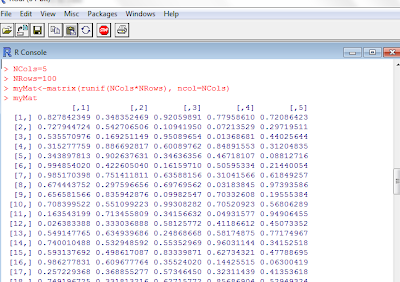
Now,  you will need a data matrix. I don't have a good one on hand, so I'm going to make a random one

so you see, I told it to make the number of columns as "6" (Ncol = 6), the number of rows as 100 (Nrow=100), then I named my matrix "myMat" and ran it for the size of Ncol* Nrow where the number of columns is Ncol.

Now I want to load up that package we just installed. Take a look back at picture 1 if you are confused, but go to Packages > Load Package, and you should see "FactoMineR" on there. Just click it and you'll see some stuff in the command prompt.

Okay, you got this.

Now, just tell it

result = PCA(myMat)

and you will get this:

Because myMat was drawn from a random distribution, there aren't any correlations amongst my vectors. Nonetheless, this is a neat tool, and that graph on the left was apparently pretty cool to people at AGU. I hope you can use this tip for your own presentations for easy and fun PCA!

Coordinates from arrays and surfing in MatLab

So I've been embarking on a mission to make a good, conceptual model of hill slope ecosystem processes that define productivity. I've got a model that describes some of these processes already and it's pretty useful, but right now playing with it is pretty hard because it invokes a lot of details that are beyond the current (basic) scope of what I'm thinking of.

So I decided that I would take the pre-processed DEM file from that model (processed to allow downhill percolation) and specifically the part cut to the boundaries of my watershed, and start to play with it.

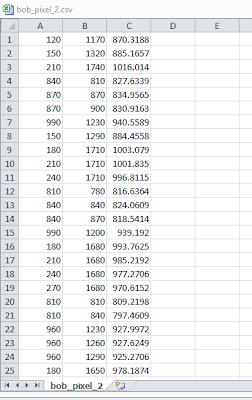
One challenge was that I essentially had the data in a format that was 3 vectors (columns) of x-axis location, y-axis location, and z-axis locations. I had no idea how to process this, so I asked my husband who wrote me a script and then kindly explained it to me.

Here's the original file:

My file is called "ws1_elev" which you can see below how it is imported here:

so first, he created two variables, "data" which is essentially the same as "ws1_elev" and "N" which is the length of the data (I believe it was something like 1151 rows long).

Now, my x and y coordinates were on a 30 x 30 m scale, and since I wanted to look at this as a picture, that would not be convenient for here. I would have just one point every 900 square meters. So we divided the x and y coordinates by 30 by saying:

data( : , 1 : 2) = data ( : , 1 : 2) / 30 + ones (length (data) , 2) ;

in short, in the new matrix "data", all rows (: ,) of the first two columns (1 : 2) are the same as those rows divided by 30 ( /30). We then add "one" to every unit in the second column because otherwise many of these units would be "0" and MatLab does not like 0's in its arrays.

Now, we want to tell it to understand that these first two columns are actually coordinates. So here's the brilliance,  create a matrix of zeros as big as the maximum length in columns 1 and  2 (essentially think of this as making a piece of grid paper as big as your coordinates) 

A = zeros (max (data (: ,1)), max(data(:,2)));

now, for every account in your original matrix (there are N of them)

for i = 1:N 

A(data(i,1), data(i,2)) = datai3);

end

What is this doing? I didn't know, so he explained, and now I will share...
Well think of if you had a matrix in Matlab named "B." B is a matrix of random numbers drawn from the normal distribution:

Now, if you wanted to look at that component there, -0.1935, you see that, it's in the 2nd row and second column, so it's coordinates (location) are (2,2). You are calling it from "B" so call it B(2,2)

So that's what you are doing here, you are saying that the matrix A is defined by coordinates at data(:,1) and data (:,2). Furthermore, those coordinates have a specific "z-value" associated with them (in this case, it's ACTUALLY a z-value, elevation) which is stored in data (:,3). Two birds with one stone!

Now, I want to look at this matrix. And by look at it I don't mean just look at a giant array of numbers. I want it to look nice. I could use Plot3 and look at the three columns of "A" but that's just going to look bad. So instead, we use "surf"-- which stands for surface. If it looks like crud add "shading interp" which will make it colorful and nice.

So here's the whole program, and you can see "surf (A) " at the end. Figure 1 just means that it's in figure (1) (there are more than 1 figures in this program) and clf means (clear the last figure). Okay, so what's the result?

Okay so it's not perfect, but it's great to show that the file came in right and the topography looks correct.

Well that's it for now!

Statistics in MatLab

For a long time, I was a dualist scripter, in other words, I believed in using MatLab to do algebra things and R to do statistical things. Of course, when it came to stuff like regressions, histograms, etc., there was some overlap, but if the test was, well pretty much anything other than a x to y or polynomial fit, I was using R. And if the matrix needed even one eigenvalue decomposition, I was using MatLab.

One day it came to pass that I learned about the great help on MatLab, which looks like this online

Or on your computer, it can be accessed by saying:

> help NAME_OF_FUNCTION_YOU_ARE_INTERESTED_IN

Of course you will say the actual name of that function, not NAME_OF_FUNCTION_YOU_ARE_INTERESTED_IN

for example, my personal favorite, the kruskal-wallis test, which can be used with non-normal distributions to ask the question "are these samples from the same distribution?" (or distributions with equal medians...)

In short, MatLab does have statistics! And this is great when, like we have been working on, we have massive files to simulate data that is a pain in the ba-donk-a-donk to export. Why export to R to run many rank-sum tests and KS tests when you could do this in MatLab?

Now best,what if you've got a test that you need, but egads, it's not already in MatLab? For example, for a while I was thinking I needed to use Royston's test for multivariate normality. It later occurred to me that in my particular situation I could use the KS test, but as you can probably guess, Royston's test isn't one of the tests commonly found in MatLab. NO FEAR.

 Smart people out there exist who have written scripts to do this, JUST FOR MATLAB. Simply "google" the test you want and "MatLab" and you'll probably find it. I found Royston's test here.

Now to use this test you need to be able to "call it" in MatLab. So go ahead and save the file, a zip-file. When you extract that file, make sure you save it somewhere convenient, preferably in your matlab directory. You might have, for example a place called:

C:/ProgramFiles(x86)/MatLab

you could save your file in a New Folder named "RoystonMultivariate"

C:/ProgramFiles(x86)/MatLab/RoystonMultivariate

Now remember the tips I gave you in the last post about set path? If not, scroll down and review. You'll want to set that a path to the file: C:/ProgramFiles(x86)/MatLab/RoystonMultivariate that you just made. Now if you read the file documentation (which can also now be found by simply typing help roystest at the command prompt, you'll know how to set up your file to read).I think it really helps to use something like this:

[p,h,stats] = roystest(dataset);

that way you can ask for feedback like "p" (p-value), "h" (hypothesis, accept or reject) and "stats" (detailed read out).

Well, that's it for today.

importing data into MatLab

My biggest loathing in scripting is importing data. I hate it. So today I'm going to tell you how to do it in Matlab, nice and easy.
1. go to the file menu, and you will see a nice button that says Set Path (you'll see it, click file)

2. You will see an add folder option. Choose a folder that you want to keep stuff in. There's no penalty to too many folders, so I recommend making a new one for every new big project that you do (i.e. "biomass", "protein interactions," etc.)

As you can see my computer user name is Sparky, after my middle name.

3. Now you will be ready to go! Make sure you've made some files that you want to put information in. Now open up your program. Let's say you have a file named real_heigh_hist.csv you want to import (it's a nice little matrix or something, with no titles, of course, because Matlab hates titles)

4. In the MatLab prompt in your script, say:

FILE = importdata('real_heigh_hist.csv',',');

That means-- pull in this file called real_height_hist.csv, and that he items are separated by commas (csv-- comma separated values)

after you've done that for as many FILES as you want (hint: label them FILE, FILE2, FILE3, FILE4), then you will want to rename them something meaningful, like "height_hist"

Now, save your file as something nice and open it in Matlab's editor. Tada! You can call your variable (height_hist) or you can add more information to your script and have fun. 

*note: some people may find this oversimplistic-- but I know the biggest barrier for me learning to script was importing files.